ABSTRACT

Our project was born out of curiosity for the handcraft of pottery wheel throwing, one of the most tactile and oldest techniques for making. In particular, we were intrigued by the individuality of each pot, where the marks of the maker are present in each curve and ridge of the final product. We wanted to learn from craftspeople, understanding that even though a master craftsperson knows their trade-in and out, no two pots are ever the same.

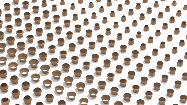
Parameter space of generated pots using our GH generative script

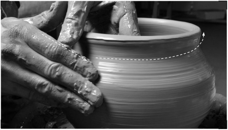
Image shows the process of creating pots using wheel throwing

Our first step was to learn from a potter, whereby we filmed her throwing several pots and began to understand the process of throwing. With a stable central axis, the wheel rotates at different speeds which allows the potter to exert forces at a particular section of the pot which then transforms the full geometry. The forces are located both on the inside and outside of the pot and work together as they simultaneously morph and stabilize the lump of clay. We were able to abstract this process into forces applied to a rotating central mass. With this clear, we endeavored to create a parametric simulation script, from which we would extract data and train two AI models: One that could predict geometry based on forces, and a second that could predict forces based on geometry. Our final goal was to create a process that could eventually be trialed with robotic fabrication.

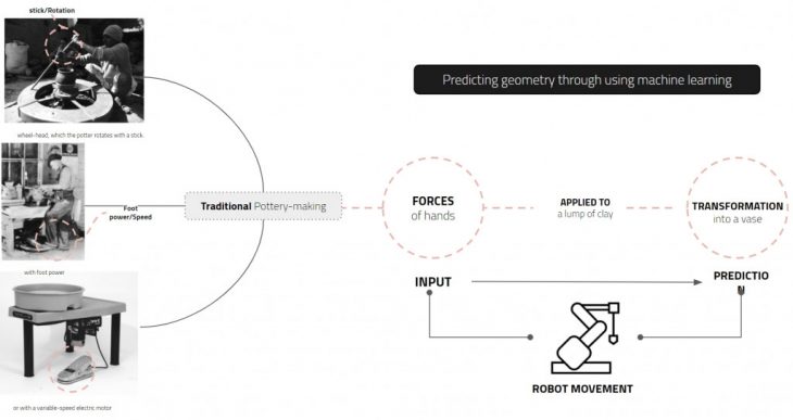
GENERATIVE PROCESS

In order to simulate the wheel throwing process, we created a central cylinder that was converted into a 3D point cloud. This cloud was rotated along a central axis, and two forces, force a and force b, were applied to it in a variety of ways. The forces had a location, a rotation value, a friction value, as well as a length, and altered the point cloud as they interacted with it. 

This was a generative process, where the rotation speed and number of rotations were equally important as the direct interaction with the forces. The final result was a mesh that acted as the simulated final pot. We repeated this action 9500 times, creating a robust parameter space from where to extract data from.

Generative process for creating digital pots

The forces and their values could be extracted from the parametric script, however, the geometry had to be extracted from the final mesh. To do this, we cut the pot in half, generating a cross-section, and placed its base at the origin of our Rhino world. Doing this allowed us to extract deviation values in the Y direction rather than having to enumerate the x, y, and z values for each point in the cross-section. As a matter of data management, this was a key element in the success of our project and was part of an iterative process that took multiple trials to fit.

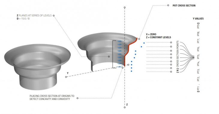
The Diagram shows how cross-sections were extracted from the generated pots.

The GIF explains what are the inputs and outputs for each generated pot

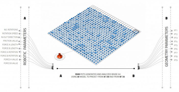
The parameter space is created by placing each generated pot on a different grid cell

The final parameter space of 9500 generated pots

THE AI MODEL AND TRAINING

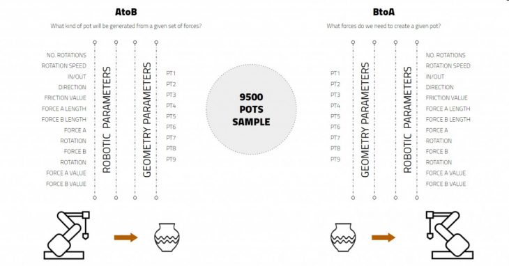
We set ourselves out to create two different AI models, one to which we would feed forces and it would predict the cross-section, essentially summarizing our parametric script to a single component and a second in which we would predict the forces needed in order to create a pot of a given geometry. We saw a major benefit in having a dual system considering that our final goal is a fabrication. 

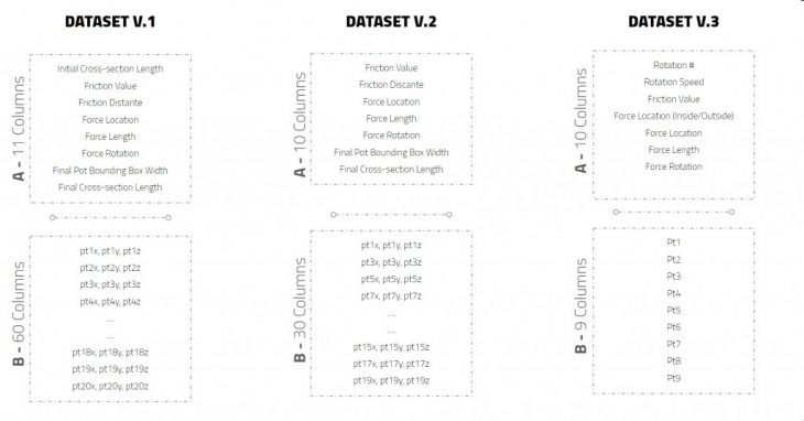
The diagram shows the dataset alternatives.

The PCA test for dataset alternatives.

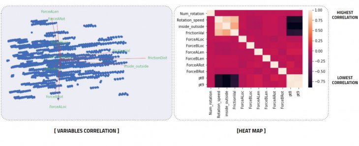
The PCA test graph shows which inputs are more important for the final predictions.

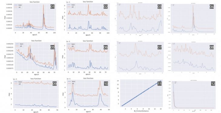
Plotting accuracy graphs for different hyperparameters.

AtoB Model

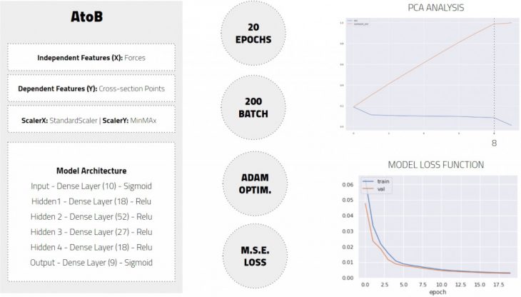
Our A to B model can predict geometries based on a given set of forces. In order to get here, we took our data through a PCA analysis that showed 8 of our variables as independent PCs and created a model architecture with 4 hidden layers that acted as a two-sided funnel. Our scalers were different from our dependent and independent variables due to the nature of their values, where cross-section points were scaled with a MinMax scaler and the forces were scaled with a StandardScaler. This first model was rather simple, as it was able to learn by training for only 20 epochs with a batch value of 200.

BtoA Model

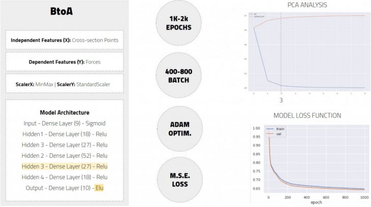
Our second model proved more complex, which resulted in an additional hidden layer in the model’s architecture, as well as a dramatic increase in the number of epochs and batch size to achieve learning. With a batch size of 400 to 800, and between 1000 to 2000 epochs our model was finally successful. Worth noting that the PCA analysis for this setup tells us that only 3 of our PCs are of importance, however, we decided to move ahead with our 9 cross-section values since we needed these in order to compare geometries.

INTEGRATION WITH GRASSHOPPER

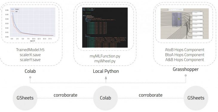
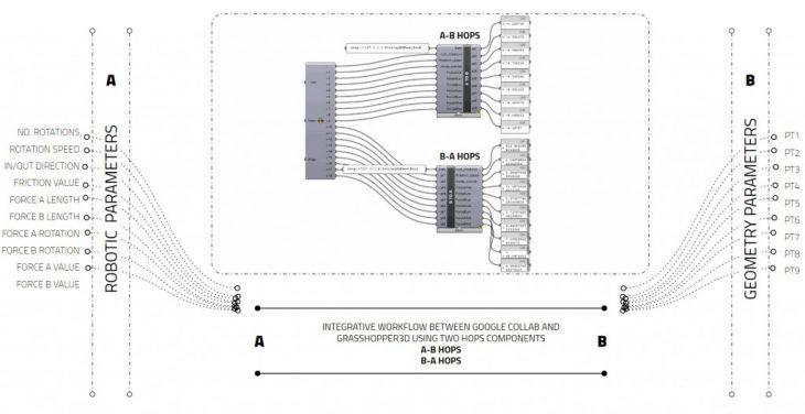
Although Grasshopper can host IronPython, the platform does not support importing libraries such as NumPy or TensorFlow. Since we were dealing with a high number of libraries, the workflow to integrate our AI models into grasshopper was done by using Hops. Hops allow us to program on a code editor such as visual studio code and connect it via a local server to the grasshopper space. This means that we can train our models in Google Colab, taking advantage of their cloud-based GPUs, and once properly trained save them as .h5 files to bring into our local machines. The hops components become hosts for the predictions given by the AI models.

FINAL PREDICTIONS

Using the Hops component we could then take advantage of visual comparison for our results – we found that accuracy and loss graphs could look good but this did not mean that the geometrical output was accurate enough. After multiple training, we managed to land at two models that indeed had an accuracy level above 90% and therefore were satisfactory. The method of geometric comparison was based on the calculation of deviation between the point values at the cross-section of the predicted and simulated pots. We found that the predicted values had a certain margin of error, but that the computational power and complexity of the parametric script were greatly reduced.

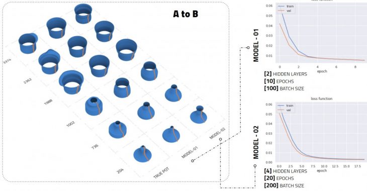
AtoB model predictions show the predicted pot on the left and the true pot on the right. The attached grasp is calculating the deviation between the predictions and the truth.

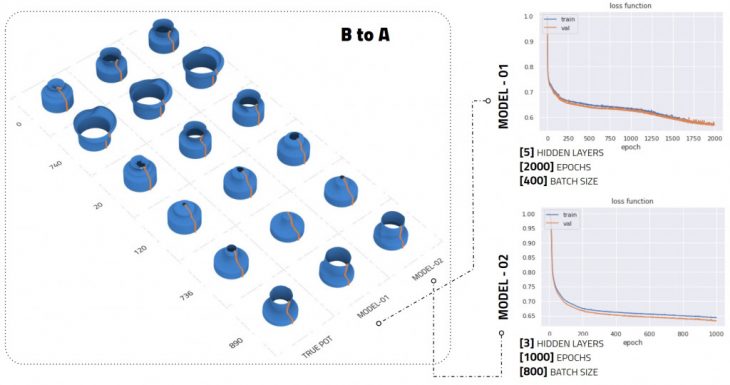
BtoA model predictions show the predicted pot on the left and the true pot on the right. The attached grasp is calculating the deviation between the predictions and the truth.

CREDITS

Imaginary Vessels is a project of IAAC, Institute for Advanced Architecture of Catalonia developed in the Master in Advanced Computation for Architecture & Design in 2020/21 by Amal Algamdey, Cami Quinteros, and Hesham Shawqy.  Faculty: Gabriella Rossi  and Illiana Papadopoulou